At Diamond Age Data Science, we make extensive use of RMarkdown and RStudio. These tools let us merge our analyses and reporting into a single framework and give our customers a way to inspect our methodology and reproduce our analyses on their own (if they wish). They also enable our customers to customize their views of our work (e.g., hiding or showing all code along with a narrative) and choose how they interact with the data (e.g., downloading tables directly to Excel, viewing dynamic plots).
But what about Python-oriented developers and data scientists who don’t want to use R? There’s a way they can also get the benefits of the RMarkdown reporting system — but it requires a bit of trickery, which I’ll show you in this tutorial.
Motivation
Alright, I admit it. I’m one of those people who dislike R. I work in Python 99.9% of the time, I’ve been programming in Python for a long time now, and I spend a lot of development time working interactively with JupyterLab. I’m delighted and productive. Could I get this productive with R? Yes. Am I motivated to do so? Not at the moment.
I am aware of the many improvements that have been made to the Python tooling in RStudio, but to me it still feels unnatural — and, though it’s much improved, it still has a way to go (in my opinion) before it is appropriate for a full-time, Python-centric, computational biology workload.
What you need to know already
To proceed through this document with ease, you should be familiar with:
This is a lot, though, and hopefully those without the full suite of knowledge above can still gain some appreciation of the system I’m going to describe.
R and Python
For many years now, the Python community has had really nice integration with R through rpy2 and the cell magic of %%R in Jupyter/IPython. I used it in both my PhD and postdoc work, as well as professionally, and it’s great. However, it has always been a pain point to create the (admittedly) beautiful reports that come almost stock with RMarkdown. Pair the narrative with the analysis possibilities of the R ecosystem, and one may wonder why more complete Python-to-R switches are not made by professionals doing this kind of work.
Recent TIOBE metrics may tell part of the story. R dropped 0.52% between 2019 and 2020 and was overtaken by (gasp) Visual Basic. (I have some cred here — the first application I wrote professionally was in Visual Basic, over 20 years ago.)
For those of you how may have not seen this R-from-Python scenario in action before, here’s a taste using IPython %%R magic in a JupyterLab notebook backed by an IPython kernel.

Briefly, you load the extension from rpy2 into the notebook, annotate a code cell with %%R, and use R as you normally would. This example uses R from Python. Functionality also exists to use a native R kernel in JupyterLab (i.e., no Python interface), but that is outside the scope of this post. More info on this type of setup can be found here.
From .ipynb to .Rmd (pain)
So, let’s set the stage: Here I am, happily developing code in JupyterLab (sometimes in %%R cells, but mostly not), and I finish my analysis. Things look great – like ROC AUC = 0.999 great – and now I need to write up the report of how all of this magic happened and why it matters to our clients. So, I begin…
- Open RStudio
- Load up our Diamond Age-branded RMarkdown (
Rmd) template - Sigh
- Begin the report
I have a choice to make. (It is one I have to make a lot.) For the sake of example, let’s pretend I did a large machine learning project on some RNA-Seq data, and analyzed the data in a JupyterLab notebook on an EC2 instance with a lot of memory and many CPUs (more than a laptop or desktop). The choice: do I put the code in the Rmd, or do I just report intermediate results? More often than not, the latter makes the most sense. Our clients often don’t have the infrastructure, expertise, or desire to duplicate the environment I’ve used to analyze their data, nor do they have the desire to take delivery of and deploy a docker image with everything installed. (There are advancements happening in this space that are exciting, however. Gigantum and CodeOcean, I’m looking at you!)
Back to the intermediate data: From the JupyterLab notebook, I write out the necessary text files generated by my analysis, and then code them up in my Rmd. I write R to pull them in, massage them, and display them nicely with our downloadableDT function. All of the text is written in RStudio as well, as the analysis is recapitulated, cell-by-Jupyter-cell, to weave and tell the analysis story. Back and forth I go, JupyterLab -> RStudio -> JupyterLab -> RStudio… until my head (and whatever is left of my soul, if such a thing even exists) hurts. There must be a better way, I tell myself.
Until about a year or so ago, I was without one. Until Jupytext.
The magic of Jupytext
I’ve been a fan of Jupytext since the moment I first saw it, using it mostly in conjunction with the percent output format to commit my otherwise unwieldy .ipynb files to git repositories as .py files with %% cell markup. Jupytext would then faithfully recreate the notebook files when cloned to a new system, and things would be back up and running quickly. Additionally, cell-level changes would be sanely represented in diffs. Sharing was also a breeze, and as long as my collaborator had JupyterLab and Jupytext set up, things would just work. Someone should give Marc Wouts 1000 stroopwafels.
Here’s something even more amazing: with a change to just one lone setting, Jupytext can write Rmd files from Jupyter notebooks running Python kernels! One day, this just clicked for me. “Hey, maybe I can get rid of all of this Rmd double-work.”
Indeed. Here’s how.
Environment setup
In order to facilitate writing this post, I chose to create a fresh (and even usable) docker image that contained what I needed to get started with this system. I leveraged the Jupyter Docker Stacks to build a base image and added some of the R packages I need to complete the demo. Feel free to take and use.
The Dockerfile
FROM jupyter/scipy-notebook:7a0c7325e470
USER root
RUN apt-get update && \
    apt-get install -y libreadline-dev libicu-dev libicu60
USER jovyan
RUN conda install -c conda-forge jupytext \
    R \
    r-tidyverse \
    r-dt \
    r-reticulate \
    rpy2 && \
    jupyter lab build
The Makefile
Building and running the environment is controlled using a Makefile, as below.
DOCKER_TAG=scipy-notebook
TEMPLATE_NAME=template.Rmd
build:
    docker build -t $(DOCKER_TAG) .
run:
    docker run -p 10000:8888 \
    -v $PWD:/home/jovyan/work $(DOCKER_TAG) \
    start.sh jupyter lab
knit:
    Rscript -e "rmarkdown::render('$(TEMPLATE_NAME)')"
I like a Makefile for this kind of thing. It’s a useful way to get things to work forever without having to memorize commands. I do this a lot, and along with my beard and colorful shoelaces, it increases my hipster cred.
Setting up your JupyterLab environment
After building your environment with the Dockerfile and the Makefile using make build and make run, you’ll be presented with a JupyterLab instance that is running on port 10000. Go there: http://localhost:10000. You’ll be presented with a screen that looks like the one below, asking you for a token or a password. In this demo, you’ll be using a token.
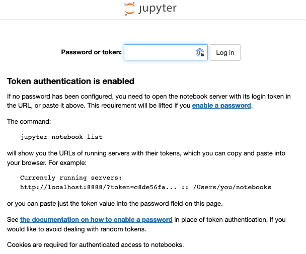
From your command line where you ran make run, you’ll find the token looking something like this:
http://127.0.0.1:8888/?token=8725da7b2c9b5a1a37986b923b1eae6c69b36426d3c6a9e2From here, you would copy everything after token= into the JupyterLab text box. Don’t get confused about port 8888 here. This is the port inside the docker container. To get to it, you’ll use the mapped port of 10000.
Go ahead and log in with the token: https://localhost:10000
Creating your notebook, template.ipynb.
After logging into the JupyterLab Interface, create a new notebook by clicking on the Python 3 icon under the Notebook section. Rename Untitled.ipynb to template.ipynb.

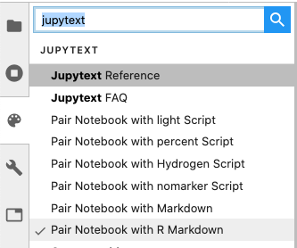
Using the command palette, associate template.ipynb with “R Markdown” as shown below.
Now, after saving the file, you should see a template.Rmd file in the File Browser.
Adding the R Markdown YAML header
Now that you have the pair of ipynb-Rmd files, we’ll be making changes manually, only to the ipynb file. This is after all, what we want to do in the first place: work in our beloved JupyterLab environment, but come out the other side with a nicely formatted html document processed from R Markdown.
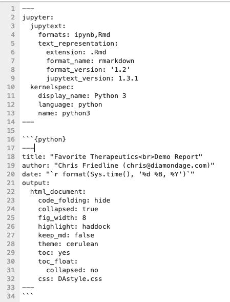
Our standard Diamond Age YAML header looks like this.
---
title: "Favorite Therapeutics<br>Demo Report"
author: "Chris Friedline (chris@diamondage.com)"
date: "`r format(Sys.time(), '%d %B, %Y')`"
output:
  html_document:
    code_folding: hide
    collapsed: true
    fig_width: 8
    highlight: haddock
    keep_md: false
    theme: cerulean
    toc: yes
    toc_float:
      collapsed: no
    css: DAstyle.css
---
There are some nice things in here. We’ve designed our own CSS to make things look snappy and we make sure our date is always correct with a bit of R code. However, if we put that into a regular cell in the notebook, as below:

What we see are two bad things:
- I can’t actually run the cell since it’s definitely not valid Python
- The paired R Markdown looks like this:
This is not what we want. What we want is for the R Markdown header YAML to be merged with the Jupytext header YAML. To do this we use a Raw Cell.
Back in the notebook, change the cell to Raw (using either the command mode keyboard shortcut, r, or using the menu above).
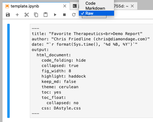
Now, after saving, you can see that the header has been merged. Is this magic? You bet it is.

Fixing up the R Markdown indenting
We discovered, as scientists who sometimes (always) write highly-indented documents, that this doesn’t play nicely with R Markdown after maybe three levels. To get around this, we use some code like the below:
<!-- script for proper TOC indenting -->
<script>
$(document).ready(function() {
  $items = $('div#TOC li');
  $items.each(function(idx) {
    num_ul = $(this).parentsUntil('#TOC').length;
    $(this).css({'text-indent': num_ul * 10, 'padding-left': 0});
  });
});
</script>
So, how the heck do we get this into the notebook (and subsequently into our Rmd)? We know we can’t use a Code cell because of the same issue we had with the header. Can we use Raw? It turns out that we can’t, because the code gets wrapped in a Python block.
```{python active="", eval=FALSE}
<!-- script for proper TOC indenting -->
<script>
$(document).ready(function() {
  $items = $('div#TOC li');
  $items.each(function(idx) {
    num_ul = $(this).parentsUntil('#TOC').length;
    $(this).css({'text-indent': num_ul * 10, 'padding-left': 0});
  });
});
</script>
```
If, however, we use a Markdown cell type, things work properly. Presumably, since Markdown is shorthand for html, this makes sense. Change the cell type to Markdown and save. Now you see this properly:

This translates to:
---
title: "Favorite Therapeutics
Demo Report"
author: "Chris Friedline (chris@diamondage.com)"
date: "`r format(Sys.time(), '%d %B, %Y')`"
output:
  html_document:
    code_folding: hide
    collapsed: true
    fig_width: 8
    highlight: haddock
    keep_md: false
    theme: cerulean
    toc: yes
    toc_float:
      collapsed: no
    css: DAstyle.css
jupyter:
  jupytext:
    formats: ipynb,Rmd
    text_representation:
      extension: .Rmd
      format_name: rmarkdown
      format_version: '1.2'
      jupytext_version: 1.3.1
  kernelspec:
    display_name: Python 3
    language: python
    name: python3
---
So far, so good. But we also need to set global knitr options in our document as per our convention. How do we do this in the notebook?
Adding R cells
As Markdown
Setting values for R cells can be done in two ways. First, we can use Markdown cells with code fencing (```), as below:

Which pairs with a proper r cell in R Markdown:
<!-- #region -->
```{r setup, include=FALSE}
knitr::opts_chunk$set(echo = F, fig.height=8, fig.width=8, message=F, warning=F, cache=F)
```
<!-- #endregion -->
As Code
If we don’t need other header information, we can also use a Code cell with %%R, which does the same thing.

This pairs with:
```{r}
library(reticulate)
use_python("/opt/conda/bin/python")
source("utilities.R")
```
Adding a header image
We also include a header image on our reports, as would any self-respecting report writer, and we have self-respect in spades. We do this with a markdown cell, as the code is technically html.

And we get that line in our R Markdown, as expected.
Let’s inspect
At this point, we have the basics in place to render the Jupytext R Markdown sibling document to html. We can do this with the make file target knit. Since we are working in the dockerized JupyterLab environment, we don’t need to leave to drop to a command line, but rather, we can use the built-in terminal. Click the + in the upper left to launch.

Change to the work directory (e.g., cd work), and run the target
make knit
If you happened to not use the naming convention above, feel free to use the Rscript command directly, with whatever name you choose.
Rscript -e "rmarkdown::render('YourSillyName.Rmd')"
Assuming everything works correctly, and it should, you should be left with a template.html (or a YourSillyName.html) file. Open that up in a browser and marvel at your accomplishment.

You’ve just written and rendered an R Markdown document in JupyterLab using Jupytext and a Python kernel. Hooray!
Finishing your report
As it turns out, our clients want slightly more information than what’s in that report, so we can go ahead and create a basic structure and write it. I’d be a terrible consultant if I gave away our secrets for free, so, please forgive this trite example.

Let’s knit it again. make knit

Better, right?
What about cell metadata?
In your R markdown, what if you wanted to not include a code cell. If you look at the previous report, you’ll see that pesky Code button in there.
The markdown you want looks like this:
```{python echo=FALSE, include=FALSE}
import pandas as pd
```
But how do you get your code cell to have that information? The answer: Cell Metadata.
Each cell has editable metadata. By default, it’s an empty JSON dictionary. Reminder, this is JSON, not Python.

To get those echo and include options in there, select the cell on the right and edit it’s Cell Metadata dictionary, as shown.

Make sure to click the check mark to embed the metadata into the cell. Once you do that, it will format the JSON. Now, when you save, you should see the translated options in the Rmd.

is now:
```{python echo=FALSE, include=FALSE}
import pandas as pd
```
This also works for thos %%R magic cells.

becomes
```{r echo=FALSE}
library(reticulate)
```
After adding those options to the code cell, make knit again and verify that your code cell button is now gone.
What about running code?
So, the whole goal of this exercise is reproducibility, right? Which means we have to run code at some point, right?
Here’s an example of how this might be done.
Consider these cells:

We created four new cells. The first is a Markdown cell with the header # Extra fun. The next two are standard python Code cells. Finally, there’s a code cell with R magic. Note that this last cell doesn’t need to be executed. It’s there only for the rendering in the report. If you don’t want to see the code cells in the report, don’t forget to set the Cell Metadata. Now, save and make knit.

Awesome, right?
Wrap-up
Hopefully, after slogging through this post (which was totally worth it, no?), you have a better understanding of the problem I wanted to try to solve: living in JupyterLab but wanting R Markdown reports.
However, this solution is not perfect. What I’ve shown in this tutorial involves a lot of nuance (and some amount of trial and error). Some cells can be executed (like the Python analysis code cells) and some can’t, and the difference between the two is not always clear. Then there’s the fact that hooking all of this up involves a lot of moving parts. It’s complex, with a high bar to entry. I’m looking forward to the day when the Jupyter publishing ecosystem catches up natively with the R publishing ecosystem — maybe then I’ll be writing shorter tutorials.
Files
Here are the files I mention in this document that I can share: